| Friday, December 7 | (Lecture #27) |
|---|
A nice fact that we will use later
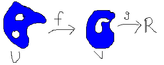
Assume the following: U and V are open sets in C, f:U-->V holomorphic and h:V-->R harmonic. What do we know about hof? If V is simply connected, then h has a harmonic conjugate, thus h is the real part of a holomorphic function (h=Re(g)). In this case gof is holomorphic, so hof=Re(gof) which is a harmonic function. The image to the right was supplied by the "scribe". Appropriate thanks are certainly due to him.
If V is not simply connected, it is still locally simply connected (just choose small balls around each point), so this is all still true locally. Since holomorphicity is a local property, the result is still true:
Proposition The composition of a harmonic function with a holomorphic function is harmonic.
Another proof of this fact is given on page 213 in the textbook (using differential operators and the Chain Rule).
Why do we care about conformal (also known as biholomorphic)
mappings?
For many reasons (or else the instructor would not spend so much time
discussing it!). Here's an important example: The Dirichlet
Problem is an important problem, which arises from many fields in
Physics (electostatics, heat flow, etc.) and in probability, etc. The
general question is: given boundary data on some open set in C, is
there a harmonic function defined inside the open set which satisfies
the boundary data?
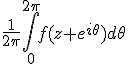
We will consider the simplest case: The function defined on the boundary is continuous and the domain is simply connected. By the Riemann Mapping Theorem (which we will not be able to prove ... please see the textbook), this domain can be conformally mapped to the unit disc. By our "nice fact that we will use later" (later being now), solving the Dirichlet problem on our open set is equivalent to solving the Dirichlet problem on the unit disc.
Solving the Dirichlet problem on the unit disc
The instructor told us that there are many ways to solve this, some
including bugs (Brownian motion), electrons ("Kelvin's Method of
Images"), and other strange ideas. Also, there is the solution as
given in the textbook, which is something like "Here is the
solution. Just compute and see that it's right" (around page 214).
Instead, we will try to find the solution ourselves.
What we know about harmonic functions:
 , therefore, since harmonic
functions are real parts of holomorphic functions, this is also true for
harmonic functions.
, therefore, since harmonic
functions are real parts of holomorphic functions, this is also true for
harmonic functions.
O.k., it's time to start solving! We are trying to define a function L
from the set of continuous functions on ![]() D1(0) to the set of
harmonic functions on D1(0). Let b be the boundary
function: b is a continuous function on
D1(0) to the set of
harmonic functions on D1(0). Let b be the boundary
function: b is a continuous function on ![]() D1(0), so by Fourier
series (since b is also in L2),
D1(0), so by Fourier
series (since b is also in L2),  almost everywhere. The solution
to the Dirichlet problem is linear in b. L also maintains limits
because by the Max/Min Principles, if b1<=b2
then L(b1)<=L(b2). So we only need to solve
for one of the terms.
almost everywhere. The solution
to the Dirichlet problem is linear in b. L also maintains limits
because by the Max/Min Principles, if b1<=b2
then L(b1)<=L(b2). So we only need to solve
for one of the terms.
 (* is convolution
on the circle).
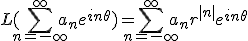
This series can be represented more nicely.
(* is convolution
on the circle).
This series can be represented more nicely.
Here is the argument, I hope without many mistakes
in algebra:
Consider
SUM-![]()
![]() r|n|ein
r|n|ein![]() .
Split it up:
.
Split it up:
1+SUM0![]() r|n|ein
r|n|ein![]() +SUM-
+SUM-![]() -1r|n|ein
-1r|n|ein![]() .
.
The first sum is a geometric series (converging absolutely and
uniformly for r in an interval [0,A] with A is less than 1. It is
rei![]() /(1-rei
/(1-rei![]() ). The second sum is
similar, and the result is
re-i
). The second sum is
similar, and the result is
re-i![]() /(1-re-i
/(1-re-i![]() ). Add these two and
get:
). Add these two and
get:
rei![]() (1-re-i
(1-re-i![]() )+re-i
)+re-i![]() (1-rei
(1-rei![]() )
)
---------------------------
(1-rei![]() )(1-re-i
)(1-re-i![]() )
)
which is, on the
bottom, 1-2rcos(![]() )+r2, and on the top is
2cos(
)+r2, and on the top is
2cos(![]() )-2r2. If we add the 1 which was also there (n=0)
we get the form of the Poisson kernel displayed in the following
result.
)-2r2. If we add the 1 which was also there (n=0)
we get the form of the Poisson kernel displayed in the following
result.
Solution to the Dirichlet Problem
If b is continuous on ![]() D1(0) then the following h is continuous on the
closed unit disc, harmonic on its interior and agrees with b on its
boundary:
D1(0) then the following h is continuous on the
closed unit disc, harmonic on its interior and agrees with b on its
boundary:  , where
A proof of this is not difficult but I really think it belongs more in
a real variables course. The Poisson kernel which appears in
the solution quoted above is a standard example of what is called an
approximate identity. Here is most of an e-mail message I sent
to Mr. Pal about "approximate
identities".
An approximate identity is an attempt (!) to have an identity for the
convolution operation.
In basic analysis , convolution is defined usually for R or for
S1 (the circle: it is easiest to think of it as [0,2Pi]).
Let me discuss only the situation on R. This may be easier. Also, for
the purposes of this message, let me use the notation I(F) for the
integral over all of R of a function F.
If f and g are functions on R, then the convolution of f*g of f and g
is defined by (f*g)(y)=I(f(y-x)g(x)). So this is an integrated product
with a shift in one of the variables. This is defined if the integral
converges, of course. If the functions are continuous with compact
support or, more elaborately, are L1 (integrable functions)
then f*g is defined almost everywhere. Indeed, if you know the
appropriate version of the Fubini Theorem, convolution and the usual
function addition make L1(R) into an algebra. Convolution
is commutative and associative. The uses of convolution are many and
varied. For example, Oliver Heaviside used it to compute with
solutions of differential equations. And it is used in, say, financial
math to compute such quantities as the "present value" of an income
stream.
In the case of L1(R) convolution does NOT have an identity
(in the sense of multiplicative identity). Maybe the easiest way of
explaining this is to mention that the Fourier transform of
L1 functions are continuous functions which -->0 at
infinity, and that the Fourier transform of a convolution is just the
pointwise product of the Fourier transforms of each of the
"factors". Then a "convolution identity" would automatically
Fourier transform to the function 1, which does not -->0 at
infinity, so there is no identity for convolution.
In certain ways, convolution CAN have an identity. Oliver Heaviside
invented and used the delta function as an identity, and formalizing
this mathematically took decades. Another path is to replace the
algebraic considerations of an identity by using an "approximate"
identity. What is this?
It is usually either a sequence or perhaps a continuously
parameterized collection of eligible functions (or in L1)
so that the limits behave like a convolution identity. So, for
example, you could ask if there is a sequence of L1
functions, fn, so that fn*g approaches g (in any
sense you might like) as n-->infinity. It may not be immediately
apparent that such sequences exist.
Indeed they do. Here is one such sequence, fairly silly: take
fn to be the function which is n on the interval [0,1/n]
and which is 0 elsewhere. Then if g is in L1,
fn*g(x)-->g(x) for almost all x. And if g is continuous,
then fn*g(x)-->g(x) for all x in R (and some weak
uniformity claims can be made). But that sequence is really not so
nice, because a rectangular graph is not smooth. There are other
sequences of approximate identities. In the context of S1
and convolution on S1, the Dirichlet kernel,
Pr(t), is an approximate identity. Here is the meaning:
Pr*g-->g as r-->1- (almost always if g is
L1 and more nicely if g is continuous). The proof of this
fact is NOT hard (and is part of the proof that we "solved" the
Dirichlet Problem: the recipe supplied gets back the boundary data as
you go towards the boundary).
I decided not to give a proof principally because the proof really is
a real variables fact, and is easiest to give when the correct limit
theorems about integrals are known. It is relatively easy to verify
that the Poisson kernel is an approximate identity. The Dirichlet
kernel, which also comes up in classical Fourier series, is also an
approximate identity, but this is somewhat more difficult to prove.
The qualities which make it easy to verify that Pr(t) is an
approximate identity are these:
i) Pr(t)>0 for all r and all t.
ii) Pr(t) eventually decreases to 0 as r increases towards
1 for t NOT equal to 0 (and here 0 and 2Pi are the same!).
iii) The total integral over [0,2Pi] is 1.
I think this is all that's required, and then the proof that we'll
solved the Dirichlet problem works out easily.
An example Dirichlet problem on the unit disc
 In fact, we can also work with boundary data in L1 and
not only continuous. For this example our boundary data is: on the
upper half circle the value is 1, on the lower half circle the value
is 0. If we stick this in our amazing formula for L(b), we get an
integral that isn't easy to understand. Instead of solving it for the
unit disc, we'll solve it for the upper half plane (remember our nice
fact from before!). By the "standard" biholomorphic mapping to the
upper half plane, we reduce the problem to finding a harmonic function
on the upper half plane such that h(x)=1 for negative reals and h(x)=0
for positive reals. We can guess what could work here: the imaginary
part of a certain branch of log will work (dividing by Pi). This is of
course a harmonic function, which is equal to arctan(y/x). Boom!
Notice that we worked backwards. Although in general
we could "solve" the Dirichlet problem in a domain by transferring it
to the unit disc and solving it there, actually here we solved a disc
problem by working in a different domain, and recognizing an obvious
solution in the other domain!
In fact, we can also work with boundary data in L1 and
not only continuous. For this example our boundary data is: on the
upper half circle the value is 1, on the lower half circle the value
is 0. If we stick this in our amazing formula for L(b), we get an
integral that isn't easy to understand. Instead of solving it for the
unit disc, we'll solve it for the upper half plane (remember our nice
fact from before!). By the "standard" biholomorphic mapping to the
upper half plane, we reduce the problem to finding a harmonic function
on the upper half plane such that h(x)=1 for negative reals and h(x)=0
for positive reals. We can guess what could work here: the imaginary
part of a certain branch of log will work (dividing by Pi). This is of
course a harmonic function, which is equal to arctan(y/x). Boom!
Notice that we worked backwards. Although in general
we could "solve" the Dirichlet problem in a domain by transferring it
to the unit disc and solving it there, actually here we solved a disc
problem by working in a different domain, and recognizing an obvious
solution in the other domain!
But this is not all! After transfering back to the unit disc, if
we square root (???) we get the solution to the Dirichlet function
given a quarter of the circle having value 1. By iterating this
process, rotating and taking limits, we solve the Dirichlet problem
for all L1 functions. Again, approximate
in L1 by using a sum of step functions. This also
works!
 The next part of the "program" is to sketch a proof of the Riemann
Mapping Theorem: that any simply connected, connected open subset of
the plane which is not all of C is biholomorphic with the unit
disc. In fact, Riemann's original proof (or suggested proof!) of this
result relied first on solving the Dirichlet problem, and deducing the
RMT from that solution. One way he considering solving the Dirichlet
Problem was imagining a boundary height (the boundary data is a
real-valued function) and then lowering a flexible "membrane" over the
data. The membrance would naturally be tight, and would try to
minimize the energy, sort of hugging the boundary data. Then (this
isn't even neat enough to require a "clearly"!) the height of the
membrane over the interior is harmonic, and is the solution to the
Dirichlet Problem. This approach can actually be understood, and does
work, but, wow, it needs (from the point of view of current
mathematics) rather a lot of work. The energy is the integral over the
interior of the norm squared of the gradient of the membrane
height. And showing that there is actually a minimizer (something that
achieves the infimum of energy) is not easy. This leads to a whole
huge area of mathematics called the calculus of variations, and
variational methods of solving partial differential equations.
The next part of the "program" is to sketch a proof of the Riemann
Mapping Theorem: that any simply connected, connected open subset of
the plane which is not all of C is biholomorphic with the unit
disc. In fact, Riemann's original proof (or suggested proof!) of this
result relied first on solving the Dirichlet problem, and deducing the
RMT from that solution. One way he considering solving the Dirichlet
Problem was imagining a boundary height (the boundary data is a
real-valued function) and then lowering a flexible "membrane" over the
data. The membrance would naturally be tight, and would try to
minimize the energy, sort of hugging the boundary data. Then (this
isn't even neat enough to require a "clearly"!) the height of the
membrane over the interior is harmonic, and is the solution to the
Dirichlet Problem. This approach can actually be understood, and does
work, but, wow, it needs (from the point of view of current
mathematics) rather a lot of work. The energy is the integral over the
interior of the norm squared of the gradient of the membrane
height. And showing that there is actually a minimizer (something that
achieves the infimum of energy) is not easy. This leads to a whole
huge area of mathematics called the calculus of variations, and
variational methods of solving partial differential equations.